.
When using ASAS-SN light curves in publications, cite both Shappee et
al. (2014) and Kochanek
et al. (2017).
WARNING: V-band (cameras ba-bh) and g-band (Cameras bi-bt)
magnitudes obtained via our interface are calculated upon query using
aperture photometry, with zero-points calibrated using APASS catalog. ASAS-SN images
have 8" pixels (~15" FWHM PSF,) so blending/crowding might be very
significant in some cases. Proceed with caution before
publishing---see "Examples" below, and also in the
Kochanek et
al. paper.
Make sure you press the "I'm not a robot" button.
DO NOT attempt to use this website
via an automated script!
Note that your search will produce a permanent http link with the light curve plot
and the data, which you can share, so you do not need to run the script again to
get the same light curve.
________________________________________________________________________________________________
Example "-3": Now also serving image subtraction data (September 2021)
Retrieved on September 7th, 2021
* Source: ASASSN-21kl (Transient, SN Ia)
* Enter right ascension: 56.125667
* Enter declination: -44.63250
* Enter number of days to go back: 160
Light curve (aperture photometry):
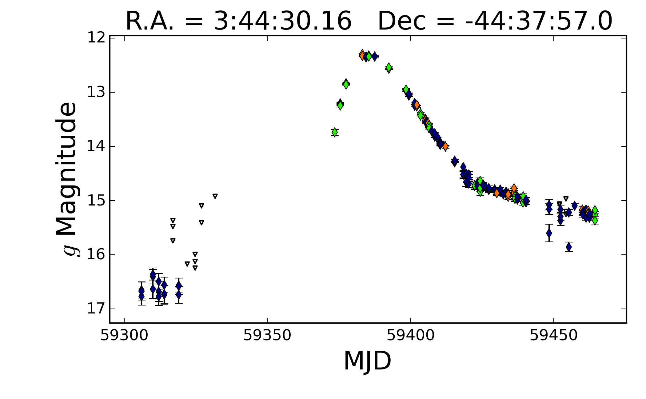 (click to enlarge).
Light curve (image subtraction with reference flux added):
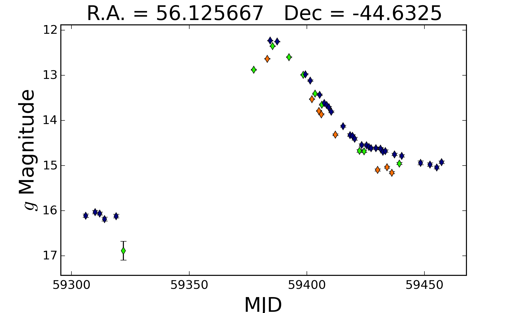 (click to enlarge).
Light curve (image subtraction without reference flux added):
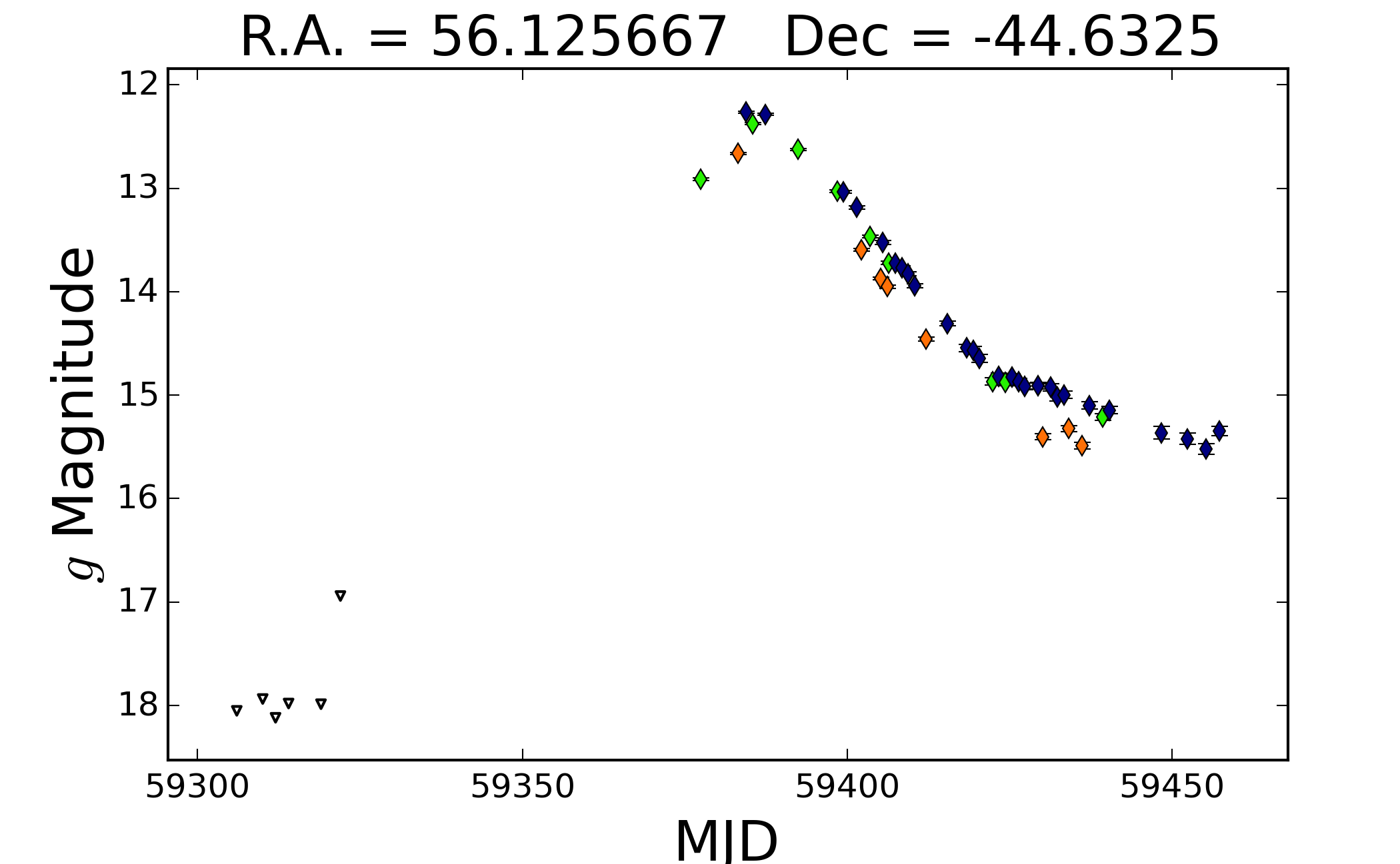 (click to enlarge).
Notes:
Aperture photometry: This does aperture photometry directly on the individual images. This is the original Sky Patrol photometry method.
Image Subtraction (reference flux added): This does aperture photometry on the coadded, image subtracted data for each epoch and then adds in the flux of the source on the reference image.
Image Subtraction (No reference flux added): This does aperture photometry on the coadded image subtracted data for each epoch but does not add the flux of the source on the reference image to the light curve.
Because the image subtracted light curves use the coadded data for each epoch (usually 3 images) while the aperture photometry light curves used the individual images, there will be fewer points but with deeper flux limits. When the reference flux is not added, the light curves will have both positive and negative fluxes because it is the change in flux relative to the reference image. Because it can be both positive and negative, these light curves can only be defined by flux and not magnitudes.
________________________________________________________________________________________________
Example "-2": Now also serving image subtraction data (September 2021)
Retrieved on September 7th, 2021
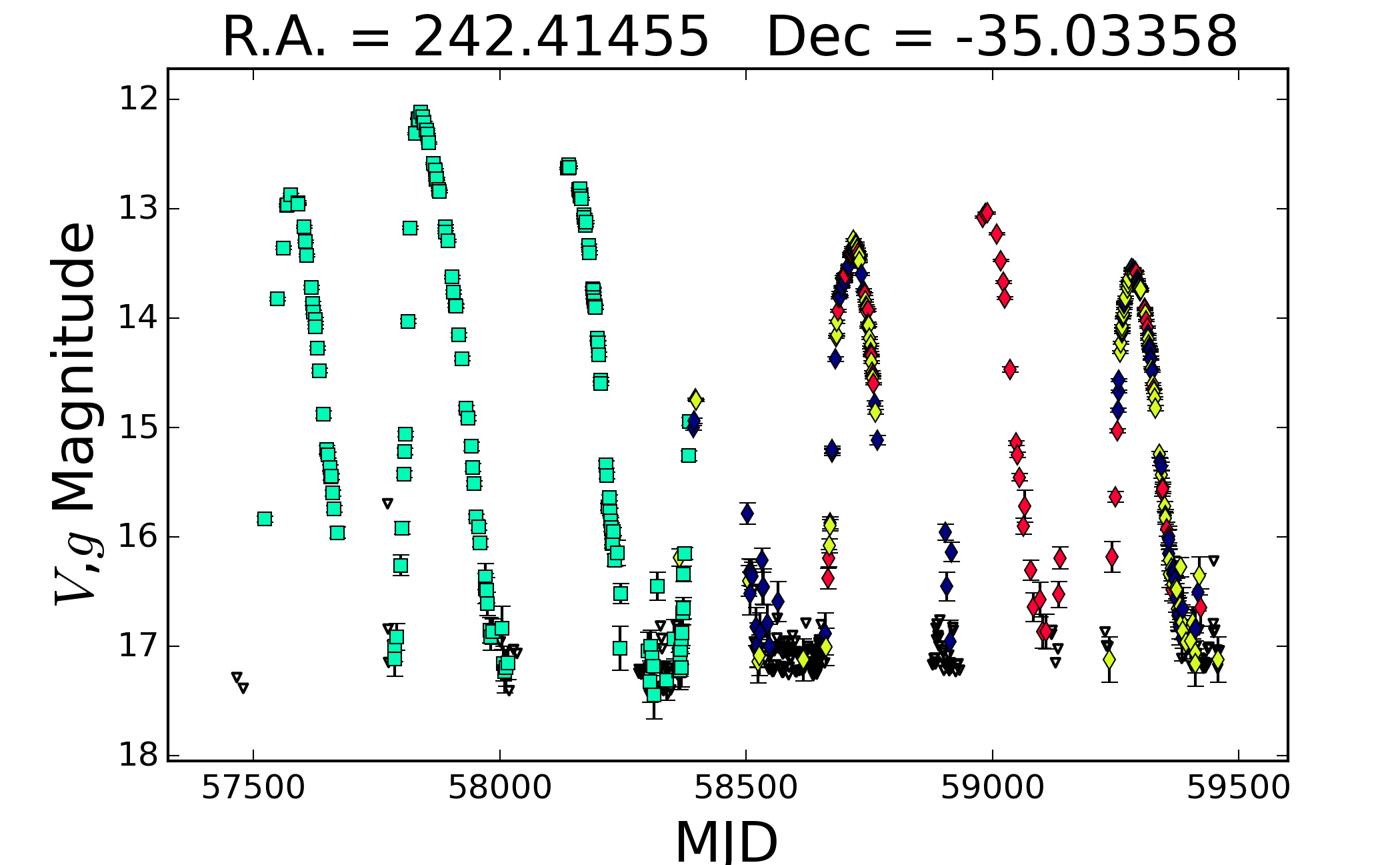
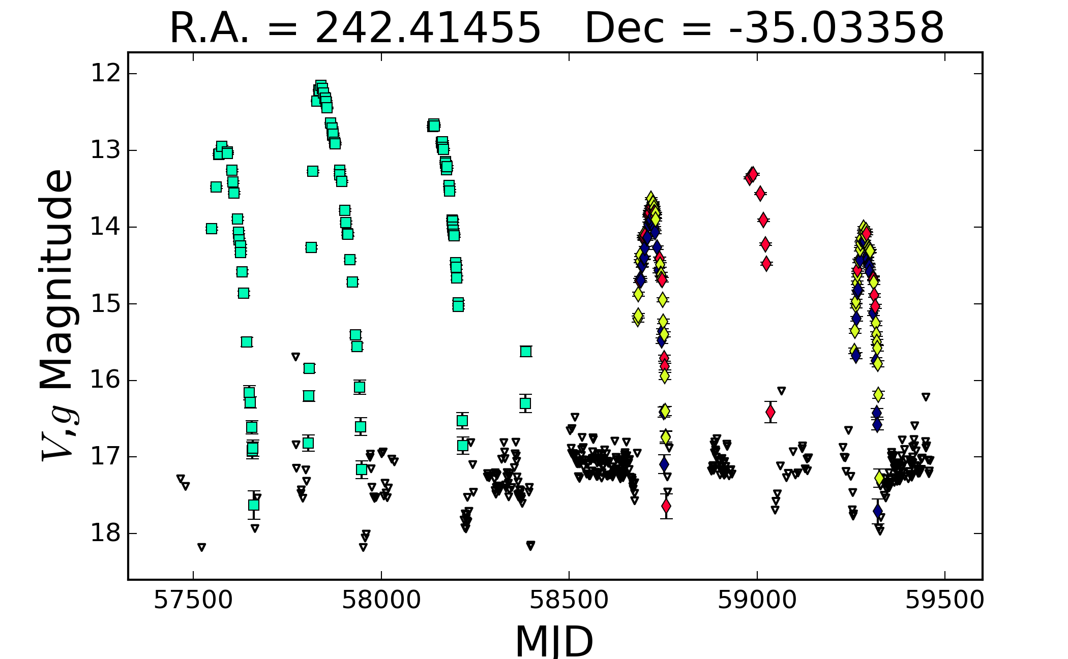
* Source: ASASSN-V J160939.56-350200.7 (Variable star, Mira)
* Enter right ascension: 242.414550
* Enter declination: -35.033580
* Enter number of days to go back: 2000
Light curve (aperture photometry):
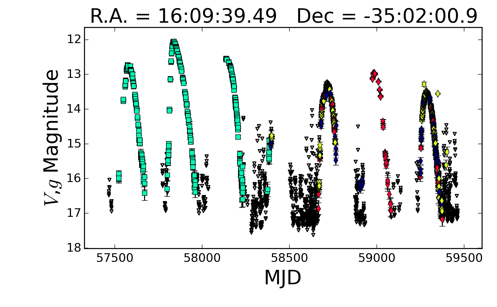 (click to enlarge).
Light curve (image subtraction with reference flux added):
 (click to enlarge).
Light curve (image subtraction without reference flux added):
 (click to enlarge).
Notes:
Aperture photometry: This does aperture photometry directly on the individual images. This is the original Sky Patrol photometry method.
Image Subtraction (reference flux added): This does aperture photometry on the coadded, image subtracted data for each epoch and then adds in the flux of the source on the reference image.
Image Subtraction (No reference flux added): This does aperture photometry on the coadded image subtracted data for each epoch but does not add the flux of the source on the reference image to the light curve.
Because the image subtracted light curves use the coadded data for each epoch (usually 3 images) while the aperture photometry light curves used the individual images, there will be fewer points but with deeper flux limits. When the reference flux is not added, the light curves will have both positive and negative fluxes because it is the change in flux relative to the reference image. Because it can be both positive and negative, these light curves can only be defined by flux and not magnitudes.
________________________________________________________________________________________________
Example "-1": Now also serving g-band data (September 2018)
Retrieved on September 24th, 2018
* Enter right ascension: 299.66840
* Enter declination: 8.37033
* Enter number of days to go back: 30
Light curve: 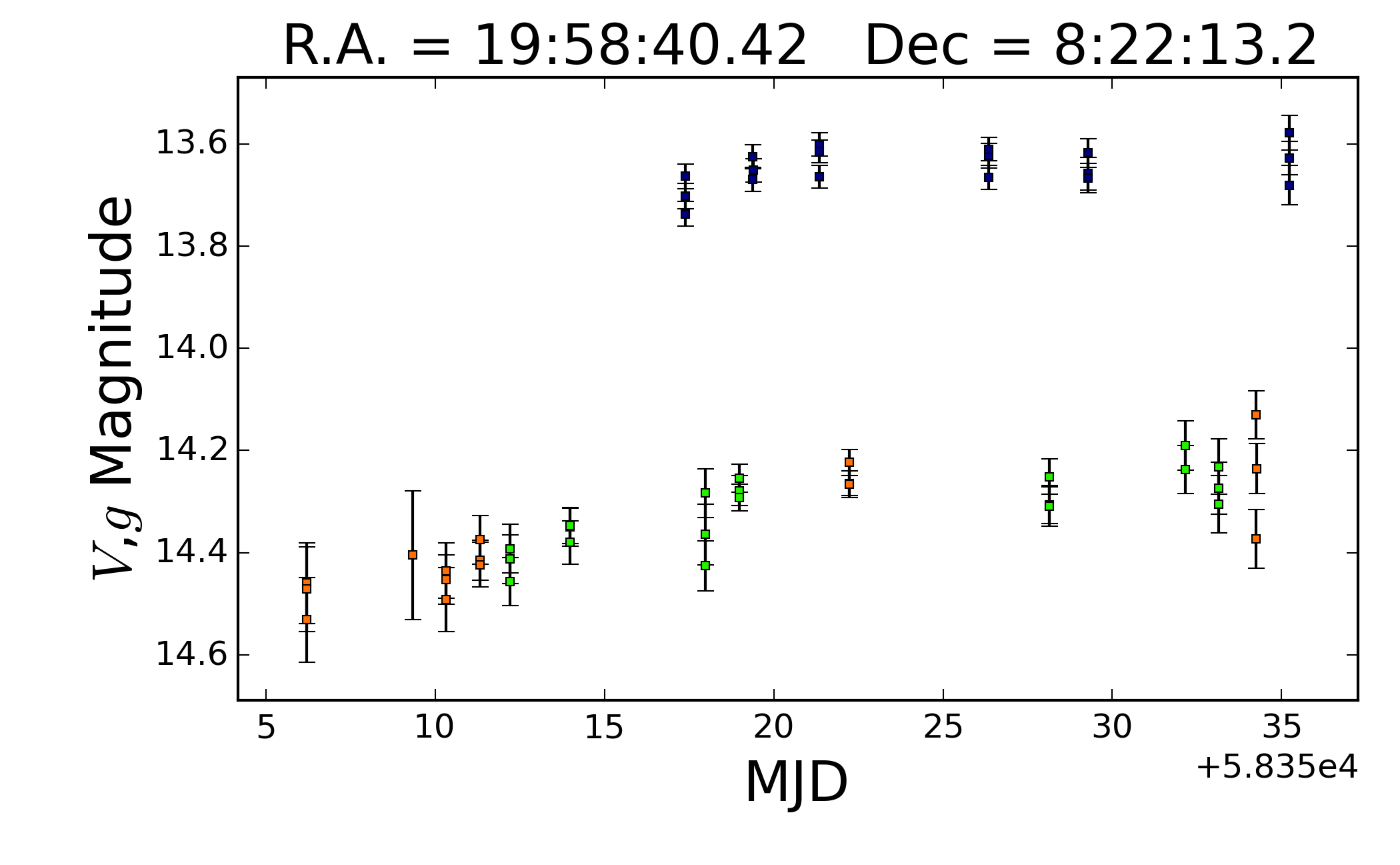 (click to enlarge).
Significant number of measurements in both V-band (top) and g-band (bottom). Return page
at this address
gives camera names, V-band is cameras "ba" to "bh", and g-band is "bi" to "bt".
________________________________________________________________________________________________
Example 0: Random spot on the sky, no data taken in the last 20 days ("behind the Sun")
Retrieved on June 19th, 2017
* Enter right ascension: 04 00 00.0
* Enter declination: +30 00 00.0
* Enter number of days to go back: 20
Output: "No data was found for this coordinate and time window."
________________________________________________________
Example 1: Random star, not known to be variable
Retrieved on June 19th, 2017
* Enter right ascension: 05 44 17.056
* Enter declination: 75 13 31.44
* Enter number of days to go back: 100
Light curve:  (click to enlarge).
Significant number of measurement (filled points with errorbars), with some upper limits. Data from one CCD only.
Note that the last data point is from April 2017, as this position is now "behind the Sun".
_______________________________________
Example 2: Random spot on the sky
Retrieved on June 12th, 2017
* Enter right ascension: 17:00:00
* Enter declination: -15:00:00
* Enter number of days to go back: 100
Light curve: 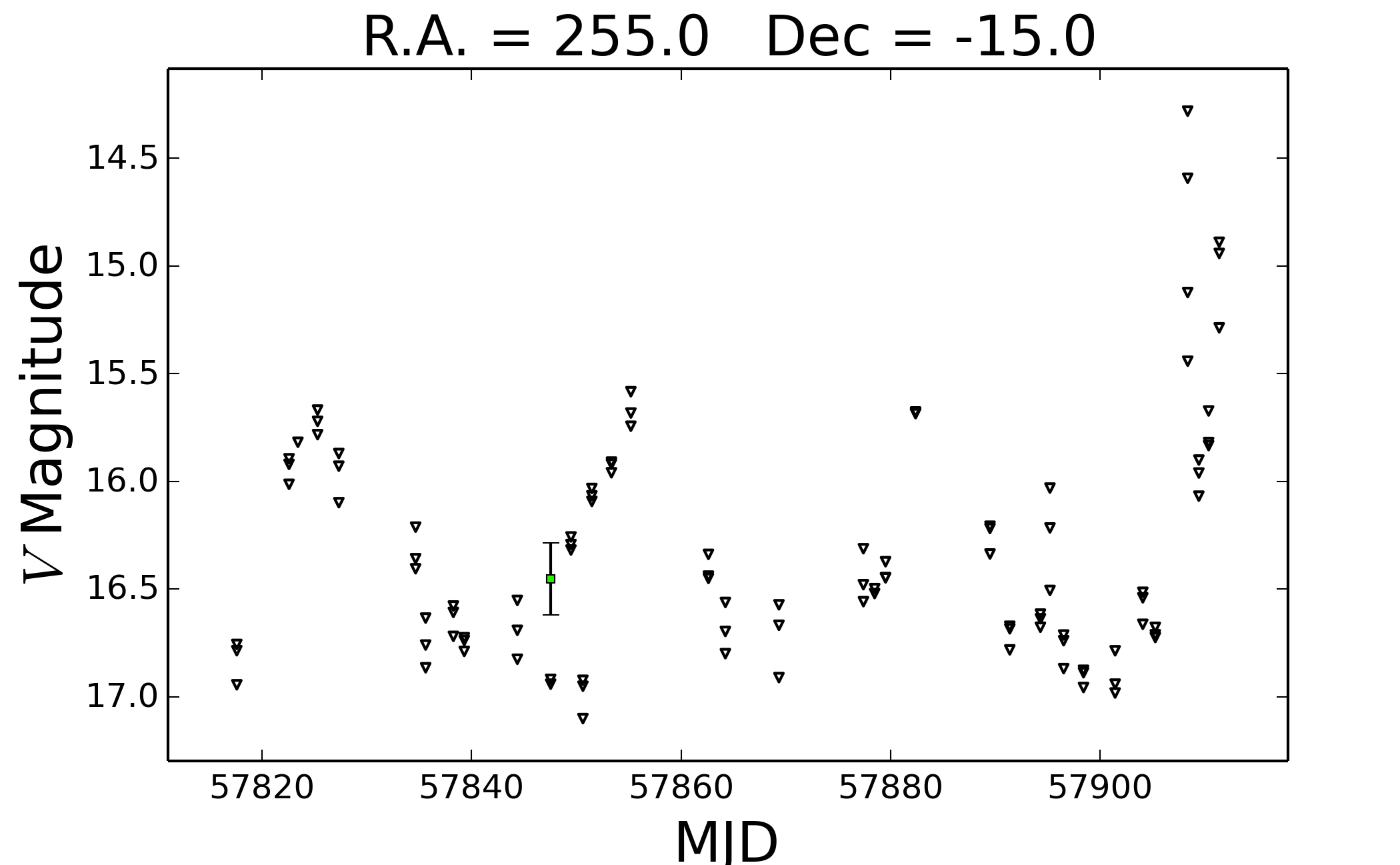 (click to enlarge).
As expected, mostly upper limits, with one (spurious) data point. One can see the influence of the Moon phase
on the depth of the photometry (but one can go deeper by co-adding 3 consecutive 90-sec exposures).
________________________________________________________
Example 3: Known Long Period Variable (V814 Sco)
Retrieved on June 12th, 2017
* Enter right ascension: 244.07975
* Enter declination: -12.78665
* Enter number of days to go back: 100
Light curve: 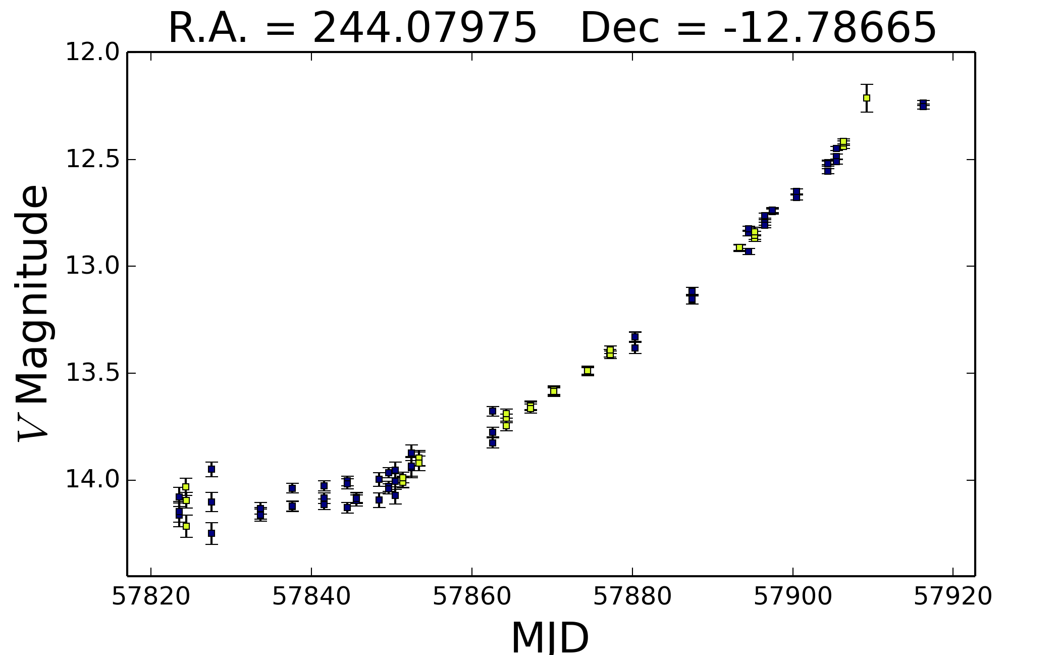 (click to enlarge).
This variable star is present in two different CCD chips ("ba" in
Hawaii and "be" in Chile), and they complement each other well. Below
we show the complete ASAS-SN light curve for the same variable (it
takes several minutes to compute the full light curve, so you should
plan accordingly). Note that the full light curve comes from 4
different CCD chips, but the majority of data are still from "ba" and
"be".
Full light curve: 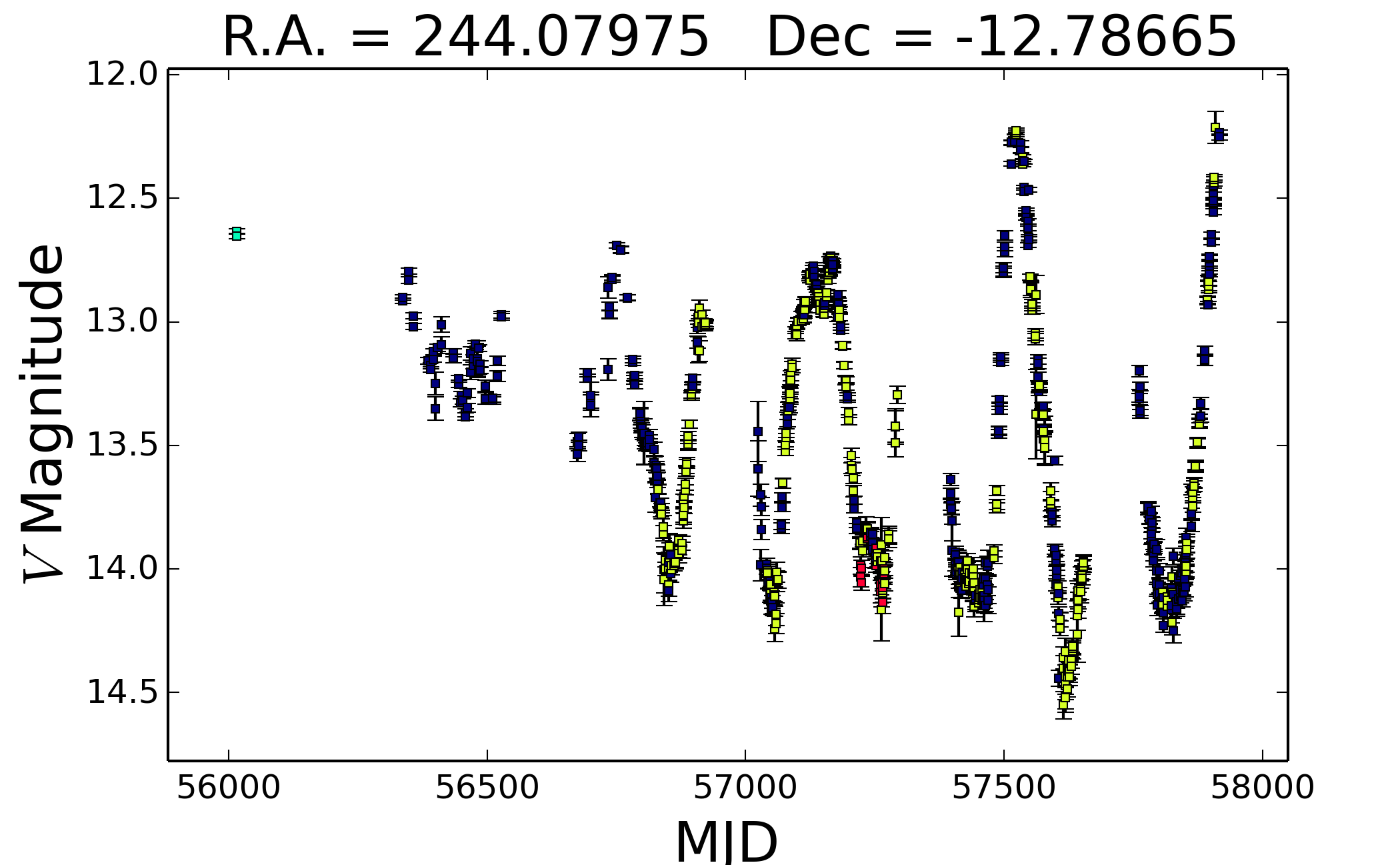 (click to enlarge).
_____________________________________________
Example 4: Galactic Nova ASASSN-16ma
Retrieved on June 19th, 2017
* Enter right ascension: 18:20:52.12
* Enter declination: -28:22:13.5
* Enter number of days to go back: 1000
Light curve: 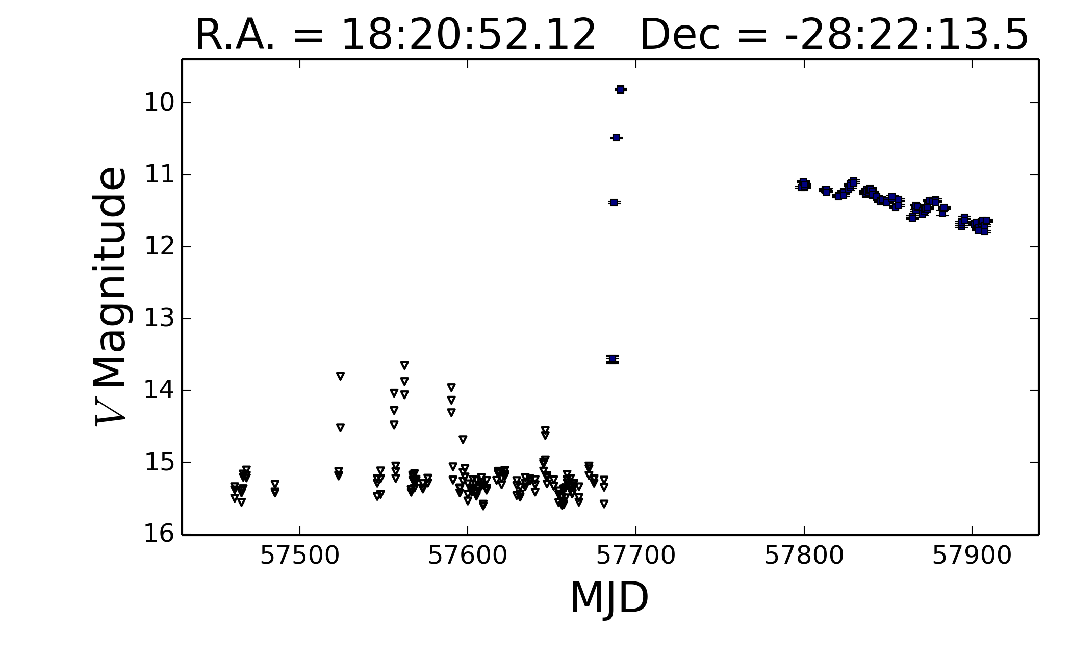 (click to enlarge).
We started observing the entire Galactic plane in 2016, hence shorter
coverage here. You are first seeing a number of upper limits (less
deep in the Galactic plane), followed by the nova caught still on the
rise. After that there is the seasonal break (field too close to
the Sun), with the nova still present in our data right now (June
2017).
____________________________________________________________________________
Example 5: Bright Galactic Cepheid VY Car, saturated in ASAS-SN data
Retrieved on June 19th, 2017
* Enter right ascension: 161.136213
* Enter declination: -57.565366
* Enter number of days to go back: 300
Light curve: 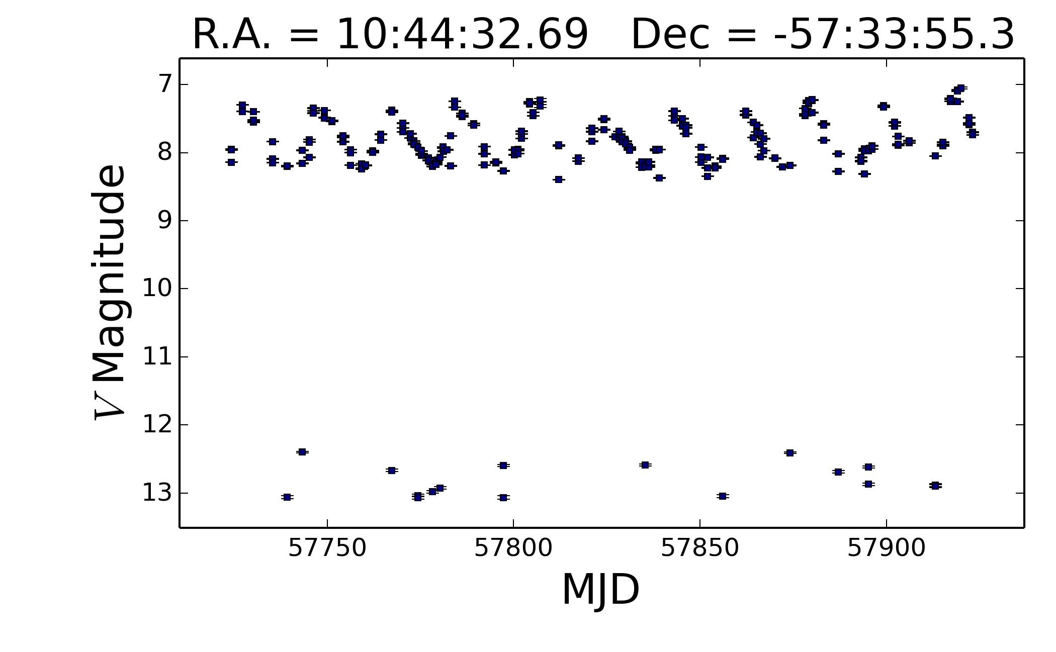 (click to enlarge).
This is an example discussed in the Kochanek et al. (2017) paper:
nominally our bright saturation limit is between 10th and 11th
magnitude (V-band, TBD for future g-band data). However, we employ a
"saturation correction" procedure, so even for object significantly
brighter than our saturation limit useful variability information can
be obtained. Indeed, one can see a clear Cepheid-like variation in the
light curve above. However, for a number of images the correction did
not work/was not applied, resulting in spurious measurements roughly
at V~13. So again, proceed with caution.
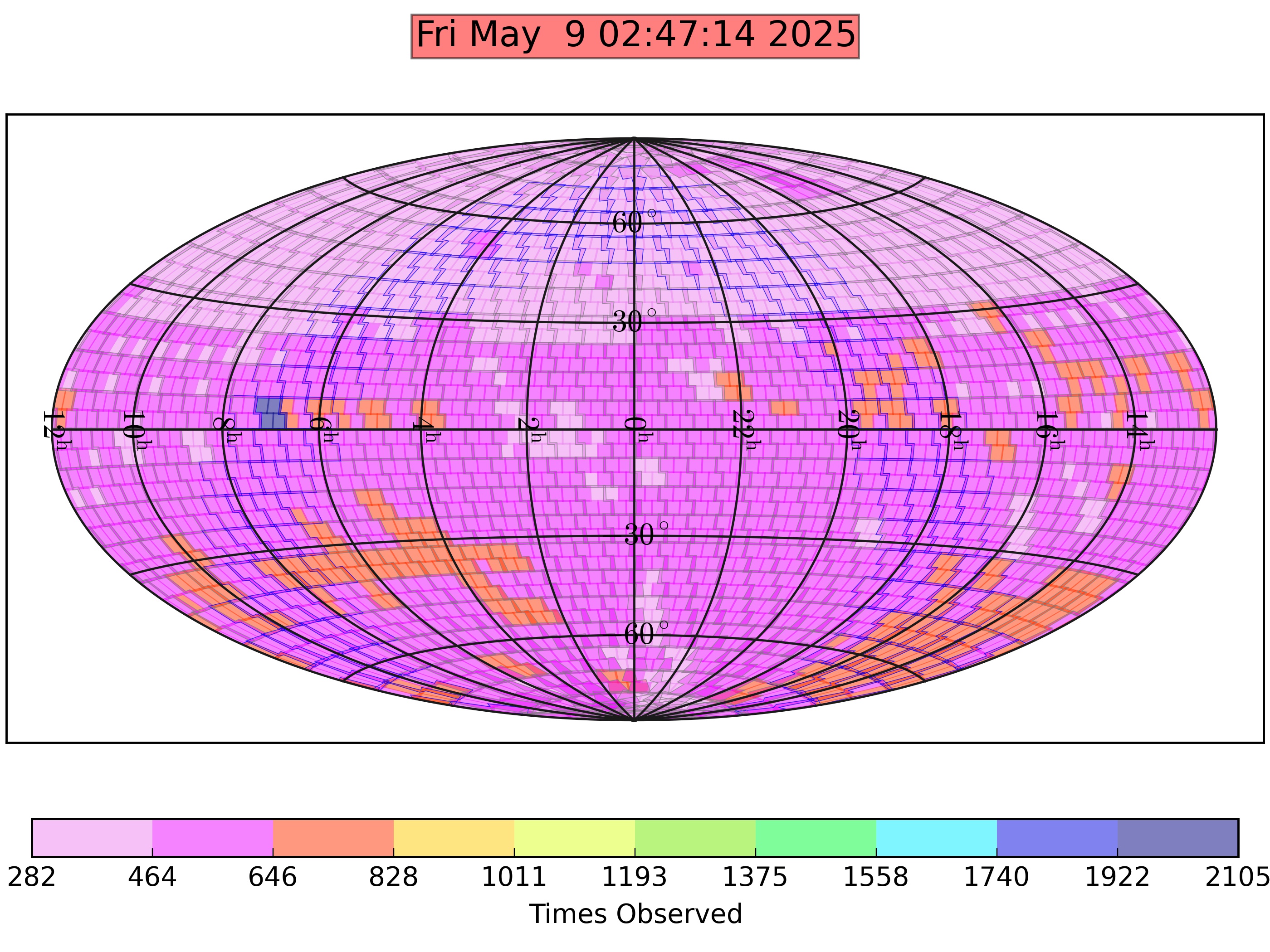
See below our sky coverage plot for the last 365 days - we are observing the entire sky!
If you have questions/comments/suggestions, e-mail Josh Shields
(shields.217@osu.edu) and Kris Stanek (stanek.32@osu.edu) (but study
the examples above first).
Updated Mon Sep 24 16:30:37 EDT 2018