Astronomy 1101: Plantes to Cosmos
Todd Thompson
Department of Astronomy
The Ohio State University
Temperature and Brightness
The nature of light
Measuring brightness and inferring luminosity
- The color of a star depends on its Temperature: Red = cool, Blue = hot
- Classification of stars by spectral lines
- Spectral differences mostly due to Temperature, not composition.
- Spectral Sequence (Temperature Sequence): O B A F G K M L T
Motivation
What do we see when we look in the sky? We see daily and annual motions of the stars and planets, which we have spent the first part of this course discussing.
On a given night with the naked eye, and from a dark site, you also see thousands of stars. You immediately notice two important characteristics: they vary tremedously in brightness (some are bright and some are faint) and they vary in color (some are blue and some are red).
What do we do with this information? How do find out what stars are? How luminous they are? How far away they are? What their temperatures are?
To answer these questions, we will first discuss light itself.
Electromagnetic Radiation
All light is Electromagnetic Radiation, a self-propagating
Electromagnetic disturbance that moves at the speed of light:
c = 299,792.458 km/sec ~ 3.0x10⁵ km/s
This is about 186,000 miles per second. Note that the speed of light is the same for any wavelength or frequency of the light! That is, blue light travels at the same speed as red light.
Light can be thought of as a wave, a periodic fluctuation in the intensity of coupled electric and magnetic fields in pure vacuum. Unlike water waves or sound waves, light doesn't need a medium to "wave" in.
Like other waves, light waves have a frequency and wavelength, usually symbolized with ν (pronounced "new") and λ ("lambda"), respectively.
The wavelength and frequency of light waves are connected. Higher frequency means smaller wavelength (bluer). Lower frequency means larger wavelength (redder). This relationship between wavelength and frequency can be expressed as an equation:
c = λ ν
Since the speed of light is a constant for all types of light, this equation says that as the frequency of a light beam gets bigger, the wavelength gets smaller and vice versa.
It is also sometimes useful to think of light as a particle, which we call a
Photon. A photon is a massless particles that carry energy at the speed of light. Your eye sees photons. Photons are reflecting off your face right now. Each photon has a certain energy. Blue (short wavelength, high frequency) photons have more energy than red (long wavelength, low frequency) photons. That is, high frequency means high energy, and low frequency means low energy. To remember this, remember that it's ultra-violet light (very blue) that burns your skin because those photons have high energy.
The Electromagnetic Spectrum
The sequence of photon energies running from low energy to high
energy is called the Electromagnetic Spectrum
low energy = low frequency = long wavelength
- Examples:
- Radio Waves, Infrared
Radio telescopes often observe radiation from
galaxies with a wavelength of λ=20 cm.
Using the formula c = λ ν, this
wavelength corresponds to ν=1.5x10⁹ waves/s.
high energy = high frequency = short wavelength
- Examples:
- Ultraviolet, X-rays, Gamma Rays
Even though individual gamma rays have much higher
frequency and much higher energy than radio waves,
they still all travel at the same speed, c.
Major Divisions of the Electromagnetic Spectrum
| Type of Radiation | Wavelength Range |
| Gamma Rays | <0.01 nm |
| X-Rays | 0.01-10 nm |
| Ultraviolet | 10-400 nm |
| Visible Light | 400-700 nm |
| Infrared | 700-105 nm (0.1 mm) |
| Microwaves | 0.1-10mm |
| Radio | >1 cm |
The Visible Spectrum
This is all forms of light we can see with our eyes.
- Wavelengths: 400 - 700 nanometers (nm)
- Frequencies: 7.5x10¹⁴ - 4.3x10¹⁴ waves/second
We sense visible light of different energies as different colors.
The basic colors of the visible spectrum are defined roughly as follows,
in order of increasing photon energy:
| |
|
|
|
|
|
|
|
| Color Name |
Red |
Orange |
Yellow |
Green |
Blue |
Indigo |
Violet |
Approximate
Wavelength |
700nm |
650nm |
600nm |
550nm |
500nm |
450nm |
400nm |
You can remember the order of these colors from lowest to highest
energy using : ROY G. BIV
Note: The wavelengths given in the table above are only approximate.
Measure brightness, infer luminosity
In order to measure the brightness of an object on the sky, we count the photons received using a light-sensitive detector. These days, we use solid-state detectors like CCDs (charge-coupled device) and similar technologies, which are much more sensitive and stable than any previous technology (e.g., photographic plates).
The brightness is just how much light falls on our detector of a given size in a certain amount of time. We sometimes call this the flux received. This brightness, or flux is related to the amount of light emitted by the source, the true luminosity, by
flux or brightness = f = L / (4 π D2)
where D in this equation is the distance to the object. This equation says that as you move farther away from an object of a given luminosity, it appears fainter to your eye, or to your light-sensitive detector (camera).
An example would be a 60 Watt lightbulb. The true luminosity of the lightbulb is 60 Watts. It can appear to be a different brightness depending on whether it is 1 meter away or 1 kilometer away.
To measure the Luminosity you need the brightness and the distance. Together with the inverse square law of brightness, you can compute the Luminosity:
L = 4 π D2 f
This is then how we measure how luminous something is. We first use a detector to gather the photons and we find that we receive a certain number of photons per second. Each of these photons has a certain energy. This tells us the total energy flux we receive from the source. Once we have this flux, we assume that the source is radiating in all directions and then we multiply f times (4 π D2) and this gives us the total luminosity L.
The biggest source of uncertainty is in measuring the distance accurately. This is a perennial problem in astronomy becasue the distances are vast, and even things that are at wildly different distances can be right next to each other on the sky. So, although we can use sensitive electronic instruments and telescopes to measure the brightnesses of hundreds of millions of stars, we have good distances (parallaxes) for only a very small fraction. Only that number of stars have direct estimates of their Luminosities.
Luminosity is an important quantity for understanding how stars work, and
measuring it with accuracy is still a practical issue even in 21st-century
astronomy.
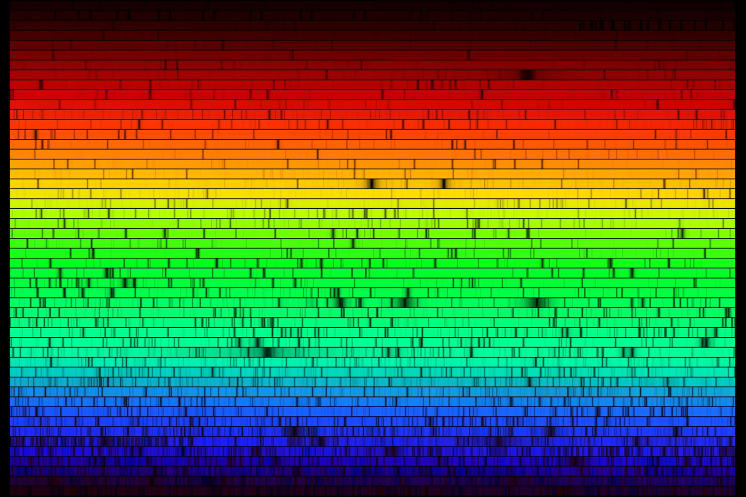
Colors of Stars
Stars are hot, dense balls of gas:
- Emit a Continuous spectrum from the lowest visible layers
("photosphere").
- Approximates a blackbody spectrum with a single temperature.
From Wien's Law we expect:
- Hotter stars appear BLUE (T=10,000-50,000 K)
- Medium-hot stars appear YELLOWISH (T~6000K)
- Cool stars appear RED (T~3000K)
More information on stellar classifications here.
Spectra of Stars
Hot, dense lower photosphere of a star is surrounded by thinner
(but still fairly hot) atmosphere.
Can we use stellar spectra to distinguish among different types of
stars?
Spectral Classification of Stars
In 1866, Fr. Angelo Secchi, a Jesuit astronomer working in Italy, observed
prism spectra of ~4,000 stars.
- Divided stars into 4 broad spectral classes by common spectral
absorption features.
[Note: Fr. Secchi was observing by eye, not using photography!]
Between 1886 and 1897, the Henry Draper Memorial Survey at Harvard
carried out a systematic photographic study of stellar spectra over the
entire sky. Effort was led by Edward C. Pickering.
- Used objective prism photography from telescopes at Harvard
and Arequipa, Peru.
- Obtained spectra of 220,000 stars.
- Hired women as "computers" to analyze spectra.
Harvard Classification System
In 1890, Edward Pickering and Williamina Fleming made a
first attempt at spectral classification:
- Sorted stars by decreasing Hydrogen absorption-line strength
- Spectral Type "A" = strongest Hydrogen lines
- followed by types B, C, D, etc. (weaker)
- Problem:
- Other lines did not fit into this sequence.
Annie Jump Cannon
In 1901, Annie Jump Cannon noticed that stellar temperature
was the principal distinguishing feature among different
spectra.
- Re-ordered the ABC types by temperature instead of Hydrogen
absorption-line strength.
- Most classes were thrown out as redundant.
After this, one was left with the 7 primary classes we recognize today,
in order:
O B A F G K M
Later work by Cannon and others added the classes R, N, and S which are
no longer in use today.
Henry Draper Catalog of Stars
Cannon further refined her spectral classification system by dividing
each class into numbered ten subclasses.
For example, type A is subdivided into:
A0 A1 A2 A3 ... A9
Between 1911 and 1924, she applied this Harvard Classification scheme to
about 220,000 stars, published as the Henry Draper Catalog.
The Harvard (or Henry Draper) spectral classification system was adopted
by all astronomers.
Two New Spectral Types: L & T
These are the coolest stars, with T<2500 K.
Discovered in 1999, they are turning up in relatively large numbers in
recent digital all-sky surveys. Because the stars are extremely cool,
they emit mostly at infrared wavelengths.
Their spectra are quite different from M stars, and 2 new spectral classes
have been proposed for them:
- L Stars:
- Temperatures ~1300-2500 K
- Spectra show strong metal-hydride molecular bands (CrH & FeH),
and neutral metals, but TiO and VO bands are nearly absent.
- T dwarfs:
- Spectra show strong bands of Methane (CH4), like
the spectrum of Jupiter.
- Most likely to be failed stars (low-mass "Brown Dwarfs") with
masses too small to ignite hydrogen fusion.
Cecilia Payne-Gaposhkin
Harvard graduate student in the 1920s. In 1925, her dissertation,
published as the book Stellar Atmospheres was
the breakthrough work in understanding stellar spectra.
- The first comprehensive theoretical interpretation
of spectral spectra.
- It was based on the then new advances in atomic physics.
Put our understanding of stellar spectra on a firm physical basis.
Her work showed for the first time that all stars were made of mostly
Hydrogen and Helium and small traces of all the other metals.
The Spectral Sequence is a Temperature Sequence
- The Differences among the spectral types are due to
differences in Temperature.
Why?
- Which spectral lines you see depends primarily on the state of
excitation and ionization of the gas.
- Excitation and Ionization are determined primarily by the
temperature of the gas.
Implications:
- Composition differences are unimportant.
- Differences in temperature are the most important factor.
Example: Hydrogen Lines
The Hydrogen absorption lines in the part of the spectrum at visible
wavelengths all arise from H atoms with the electron in first excited
state.
- B Stars (11,000-30,000 K):
- Most of H is ionized, so only very weak H lines (not much H around
with electrons to make any absorption lines)
- A Stars (7500-11,000 K):
- Ideal excitation conditions, strongest H lines.
- G Stars (5200-5900 K):
- Too cool, little excited H, so only weak H lines because the
electrons are mostly in the ground state instead of the first
excited state.
Modern Synthesis: The M-K System
In 1943, William Morgan (Chicago) and Phillip Keenan (Ohio State) added
Luminosity as a second classification parameter.
Luminosity Classes are designated by the Roman numerals I thru V, in order of
decreasing luminosity:
- Ia = Bright Supergiants
- Ib = Supergiants
- II = Bright Giants
- III = Giants
- IV = Subgiants
- V = Dwarfs
We will explain these names in a subsequent
lecture once we learn more about the physics of stars.
M-K spectral classifications of familiar stars:
- The Sun:
- G2v
- In Winter Sky:
- Betelgeuse: M2Ib
- Rigel: B8Ia
- Sirius: A1v
- Aldebaran: K5III
Why is this Important?
Spectral classification provides a way to estimate the physical
characteristics of stars by comparing their spectral features.
- Spectral differences primarily reflect differences in the temperatures
of the stellar atmospheres.
- A star's spectrum uniquely locates the star within the overall sequence of
stellar properties.
Spectral classification is a very powerful tool for understanding the physics of stars.
Supplement:
Stellar Spectral Type Mnemonics
The traditional mnemonics for remembering the spectral types are based
on the old Harvard OBAFGKM system. Some examples:
- Harvard (1920s):
- Oh Be A Fine Girl, Kiss Me
- (this is the old (tired) classic mnemonic)
However, with the addition of types L and T, we need a new mnemonic, but
no good ones have emerged...
For fun, try to make up your own mnemonic for remembering the
temperature order (hottest to coolest) of the stellar spectral types.
Updated 2014, Todd Thompson
Original version by Rick Pogge.