Astronomy 1144: Introduction to Stars, Galaxies, and Cosmology
Todd Thompson
Department of Astronomy
The Ohio State University
Lecture 9:
- Photometry & Magnitudes
- The color of a star depends on its Temperature
- Red Stars are Cooler
- Blue Stars are Hotter
- Spectral Classification
- Classify stars by their spectral lines
- Spectral differences mostly due to Temperature, not composition.
- Spectral Sequence (Temperature Sequence): O B A F G K M L T
Magnitude System
Traditional system dating from classical times, invented by Hipparchus of
Nicaea, c. 300BC.
Rank stars into "magitudes": 1st, 2nd, 3rd, etc., as follows:
1st magnitude stars are brightest stars,
2nd magnitude stars are the second brightest,
and so forth.
The faintest stars visible to the naked eye are 6th magnitude.
Qualitative ranking. Not quantitative.
Note that Magnitudes defined in this way are
measures of the relative brightnesses
of stars.
Modern Magnitude System
The modern system of magnitudes defines them as follows:
- 5 steps of magnitude = factor of 100 in brightness
- Bigger magnitude = fainter star.
- The standard of brightness is the star Vega (0th magnitude)
Examples:
- 10th mag star is 100x fainter than a 5th mag star.
- 20th mag star is 10,000x fainter than a 10th mag star.
- Faintest stars measured this far are approximately 30th magnitude.
Unlike the qualitative system of Hipparchus, the modern magnitude system
defines the standard of brightness as the bright star Vega (brightest
star in the summer constellation of Lyra), and precisely defines the
interval of magnitude.
Flux Photometry
Count the photons received from a star using a light-sensitive
detector:
- Photographic Plates (old-school: 1880s to 1960s)
- Photoelectric Photometer (photomultiplier tube: 1930s to 1990s)
- Solid State Detector (e.g., photodiodes or CCDs)
We now use solid-state detectors like CCDs and similar technologies.
These detectors are far more sensitive
and stable than any previous technology.
Calibrate the detector by observing a set of "Standard
Stars" of known brightness. This is important because
on any given day the amount and quality of the light through
the atmosphere can change significantly.
Measuring Luminosity
To measure the Luminosity of a star you need
- the Apparent Brightness (flux) measured via photometry, and
- the Distance to the star measured in some way (e.g., parallax)
Together with the inverse square law of brightness, you can compute
the Luminosity:
L = 4 π D2 f
This is then how we measure how bright something is. We first use a detector to gather the photons and we find that we receive a certain number of photons per second. Each of these photons has a certain energy. This tells us the total energy flux we receive from the source. Once we have this flux, we assume that the source is radiating in all directions and then we multiply f times (4 π D2) and this gives us the total luminosity L.
As usual, the biggest source of uncertainty is in measuring
the distance accurately.
Practical Issues
In practice, we can use sensitive electronic instruments and photometry
to measure the apparent brightnesses of many hundreds of millions of
stars.
But, we have good distances (parallaxes) for only a very small
fraction: about 100,000 stars.
- Only that number of stars have direct estimates of their Luminosities.
- Since Luminosity depends on distance squared, small errors in
distance are effectively doubled (a 10% distance gives a 20%
luminosity).
Luminosity is an important quantity for understanding how stars work, and
measuring it with accuracy is still a practical issue even in 21st-century
astronomy.
Colors of Stars
Stars are hot, dense balls of gas:
- Emit a Continuous spectrum from the lowest visible layers
("photosphere").
- Approximates a blackbody spectrum with a single temperature.
From Wien's Law we expect:
- Hotter stars appear BLUE (T=10,000-50,000 K)
- Medium-hot stars appear YELLOWISH (T~6000K)
- Cool stars appear RED (T~3000K)
More information on stellar classifications here.
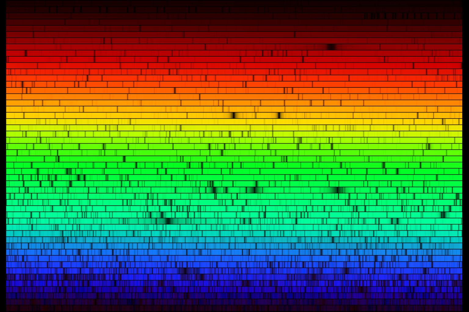
Spectra of Stars
Hot, dense lower photosphere of a star is surrounded by thinner
(but still fairly hot) atmosphere.
Can we use stellar spectra to distinguish among different types of
stars?
Spectral Classification of Stars
In 1866, Fr. Angelo Secchi, a Jesuit astronomer working in Italy, observed
prism spectra of ~4,000 stars.
- Divided stars into 4 broad spectral classes by common spectral
absorption features.
[Note: Fr. Secchi was observing by eye, not using photography!]
Between 1886 and 1897, the Henry Draper Memorial Survey at Harvard
carried out a systematic photographic study of stellar spectra over the
entire sky. Effort was led by Edward C. Pickering.
- Used objective prism photography from telescopes at Harvard
and Arequipa, Peru.
- Obtained spectra of 220,000 stars.
- Hired women as "computers" to analyze spectra.
Harvard Classification System
In 1890, Edward Pickering and Williamina Fleming made a
first attempt at spectral classification:
- Sorted stars by decreasing Hydrogen absorption-line strength
- Spectral Type "A" = strongest Hydrogen lines
- followed by types B, C, D, etc. (weaker)
- Problem:
- Other lines did not fit into this sequence.
Annie Jump Cannon
In 1901, Annie Jump Cannon noticed that stellar temperature
was the principal distinguishing feature among different
spectra.
- Re-ordered the ABC types by temperature instead of Hydrogen
absorption-line strength.
- Most classes were thrown out as redundant.
After this, one was left with the 7 primary classes we recognize today,
in order:
O B A F G K M
Later work by Cannon and others added the classes R, N, and S which are
no longer in use today.
Henry Draper Catalog of Stars
Cannon further refined her spectral classification system by dividing
each class into numbered ten subclasses.
For example, type A is subdivided into:
A0 A1 A2 A3 ... A9
Between 1911 and 1924, she applied this Harvard Classification scheme to
about 220,000 stars, published as the Henry Draper Catalog.
The Harvard (or Henry Draper) spectral classification system was adopted
by all astronomers.
Two New Spectral Types: L & T
These are the coolest stars, with T<2500 K.
Discovered in 1999, they are turning up in relatively large numbers in
recent digital all-sky surveys. Because the stars are extremely cool,
they emit mostly at infrared wavelengths.
Their spectra are quite different from M stars, and 2 new spectral classes
have been proposed for them:
- L Stars:
- Temperatures ~1300-2500 K
- Spectra show strong metal-hydride molecular bands (CrH & FeH),
and neutral metals, but TiO and VO bands are nearly absent.
- T dwarfs:
- Spectra show strong bands of Methane (CH4), like
the spectrum of Jupiter.
- Most likely to be failed stars (low-mass "Brown Dwarfs") with
masses too small to ignite hydrogen fusion.
Cecilia Payne-Gaposhkin
Harvard graduate student in the 1920s. In 1925, her dissertation,
published as the book Stellar Atmospheres was
the breakthrough work in understanding stellar spectra.
- The first comprehensive theoretical interpretation
of spectral spectra.
- It was based on the then new advances in atomic physics.
Put our understanding of stellar spectra on a firm physical basis.
Her work showed for the first time that all stars were made of mostly
Hydrogen and Helium and small traces of all the other metals.
The Spectral Sequence is a Temperature Sequence
- The Differences among the spectral types are due to
differences in Temperature.
Why?
- Which spectral lines you see depends primarily on the state of
excitation and ionization of the gas.
- Excitation and Ionization are determined primarily by the
temperature of the gas.
Implications:
- Composition differences are unimportant.
- Differences in temperature are the most important factor.
Example: Hydrogen Lines
The Hydrogen absorption lines in the part of the spectrum at visible
wavelengths all arise from H atoms with the electron in first excited
state.
- B Stars (11,000-30,000 K):
- Most of H is ionized, so only very weak H lines (not much H around
with electrons to make any absorption lines)
- A Stars (7500-11,000 K):
- Ideal excitation conditions, strongest H lines.
- G Stars (5200-5900 K):
- Too cool, little excited H, so only weak H lines because the
electrons are mostly in the ground state instead of the first
excited state.
Modern Synthesis: The M-K System
In 1943, William Morgan (Chicago) and Phillip Keenan (Ohio State) added
Luminosity as a second classification parameter.
Luminosity Classes are designated by the Roman numerals I thru V, in order of
decreasing luminosity:
- Ia = Bright Supergiants
- Ib = Supergiants
- II = Bright Giants
- III = Giants
- IV = Subgiants
- V = Dwarfs
We will explain these names in a subsequent
lecture once we learn more about the physics of stars.
M-K spectral classifications of familiar stars:
- The Sun:
- G2v
- In Winter Sky:
- Betelgeuse: M2Ib
- Rigel: B8Ia
- Sirius: A1v
- Aldebaran: K5III
Why is this Important?
Spectral classification provides a way to estimate the physical
characteristics of stars by comparing their spectral features.
- Spectral differences primarily reflect differences in the temperatures
of the stellar atmospheres.
- A star's spectrum uniquely locates the star within the overall sequence of
stellar properties.
Spectral classification is a very powerful tool for understanding the physics of stars.
Supplement:
Stellar Spectral Type Mnemonics
The traditional mnemonics for remembering the spectral types are based
on the old Harvard OBAFGKM system. Some examples:
- Harvard (1920s):
- Oh Be A Fine Girl, Kiss Me
- (this is the old (tired) classic mnemonic)
- Berkeley (late `60s):
- Oh Buy A Fine Green Kilo Man
- Caltech (late `70s):
- On Bad Afternoons Fermented Grapes Keep Mrs. Richard
Nixon Smiling
- (this uses the supplementary RNS classes that are not
strictly part of the temperature sequence, and no longer used).
However, with the addition of types L and T, we need a new mnemonic, but
no good ones have emerged...
For fun, try to make up your own mnemonic for remembering the
temperature order (hottest to coolest) of the stellar spectral types.
Updated 9/2/2013 by Todd Thompson
Original version by Rick Pogge.